Training a CNN from Scratch

What will we do today?

In this post, I will show you one of the workflows to train a CNN model from scratch, where we will build a convolutional neural network capable of estimating the age and gender of a person from their facial image.

As a data source, we will use a subset of facial images extracted from the Kaggle dataset UTKFace, however, the approach is applicable to any image dataset.

For building this convolutional neural network, we will use the Keras API version 3, now integrated into Tensorflow since version 2.0.

A bit of information...

In this section, I will share some basic concepts that will help you better understand the model development.

Artificial Neural Network (ANN)

An artificial neural network is an artificial intelligence model inspired by how the human brain works. It learns from data to recognize patterns and make decisions: from classifying images to predicting trends.

Depending on the problem, there are different architectures (topologies). Here are the most commonly used and a simple explanation of when to apply them.

FeedForward Neural Network

Feedforward networks process data in one direction: input → hidden layers → output. They do not retain memory of the past, so they are ideal for classification and regression tasks with tabular data.

Example: Predicting the price of a house using features (m², rooms, location).

Recurrent Neural Network (RNN)

RNNs process data iteratively through the same network, meaning after processing the data and obtaining the prediction at the output layer, this prediction is sent to the input layer so that the new prediction is influenced not only by new data but also by the previous state of the last prediction.

Example: Forecasting time series (daily sales) where the recent past influences the future prediction.

Convolutional Neural Network (CNN)

CNNs are designed to process data with spatial structure, especially images. They use filters (convolutions) that detect local patterns such as edges, textures, and shapes, combining this data in deep layers to recognize objects.

Example: Classifying images (dog vs. cat) or detecting objects in a photograph.

In this publication, we will focus on understanding and applying convolutional neural networks through a practical example that includes Python-based code.

There are more advanced architectures such as Generative Adversarial Networks (GANs) and Transformers, widely used in image generation and language models like ChatGPT. We will not cover them in detail here, but if you want to go deeper, I recommend this article from Microsoft.

Unraveling CNNs

Convolutional neural networks (CNNs) are a special class of neural networks designed to process data with a grid structure, such as images. Unlike traditional neural networks, which are fully connected, CNNs use convolutional layers to extract hierarchical features from the input data.

CNNs are composed of several types of layers connected sequentially:

• Convolutional layers: Apply filters to the input to create feature maps.
• Activation layers: Introduce non-linearities into the model (ReLU is the most common).
• Pooling layers: Reduce the dimensionality of the feature maps.
• Fully connected layers: Perform the final classification based on the extracted features.

Convolutional layers

These layers apply filters (also called kernels) that slide over the input image to detect local patterns such as edges, textures, and shapes.

To fully understand how these filters work, we must mention the hyperparameters kernel size, padding, and stride.

Additionally, since the filter is defined as a matrix, we can imagine the filter as a grid (a small chessboard), where the width and height are the same size. Here comes the first hyperparameter: the kernel size, which defines the size of the filter.

On the other hand, as the filter moves across the image step by step, padding refers to the addition of pixels around the edges of the image. This allows the filter to also analyze areas near the border and prevents the processed image size from being reduced.

Finalmente, el stride indica de cuánto en cuánto se mueve el filtro al recorrer la imagen. Si el paso es pequeño, el filtro analiza con más detalle pero genera un resultado más grande; si el paso es mayor, avanza más rápido, resumiendo la información pero con menos precisión. En otras palabras, el stride controla el “ritmo” con el que la red examina la imagen.

All of this may sound somewhat abstract, so let's see it with some practical examples.

In this first example, we can see how the convolutional layer would work with the following hyperparameters:

• kernel size: 3x3, that is, a grid of 3 units wide by 3 units high.
• padding: same, which means no extra pixels were added around the original image.
• stride: 1, lo que indica que el filtro avanza de un píxel en un píxel al recorrer la imagen.

Well... and what happens if we try a smaller kernel size?

• kernel size: 2x2, that is, a grid of 2 units wide by 2 units high.
• padding: same, which means no extra pixels were added around the original image.
• stride: 1, which indicates that the filter advances one pixel at a time when traversing the image.

In this case, the kernel size has been reduced to 2x2, which allows capturing finer features in the image. However, this also means that the convolutional layer will have less contextual information to work with, which could affect the quality of the extracted features.

If it's not completely clear yet, here's a quick analogy: imagine you're looking at a selfie photo of your grandmother. With a larger kernel size (3x3 or bigger), you could focus on visualizing the forehead and eyes at the same time (and then other parts of the photo like the nose and mouth); whereas with a smaller kernel size (2x2) you could focus on visualizing something more specific like just the left eye of the selfie.

Did you notice the difference? With a smaller kernel size, it's possible to see the details of a more specific sector within the image, such as even noticing pores or wrinkles around the eye. However, by reducing the kernel size, contextual information is lost, such as noticing if the color of both eyes is the same; with a larger kernel you could notice this directly in one observation.

Now that we understand the importance of kernel size, let's see what happens when we modify the values of padding and stride, and how these hyperparameters influence the functioning of the convolutional layer.

• kernel size: 3x3, that is, a grid of 3 units wide by 3 units high.
• padding: 1, which means 1 extra pixel is added around the original image.
• stride: 2, which indicates that the filter advances 2 pixels at a time when traversing the image.

In this case, a padding of 1 pixel allows the filter to also analyze areas near the edges of the image. On the other hand, a stride of 2 pixels makes the filter advance faster when traversing it, summarizing the obtained information but sacrificing some precision in the details.

So what is the best configuration of these hyperparameters? 😲

The answer is that it depends on the problem you're trying to solve and the nature of the data you're working with. Experimenting with different configurations and evaluating their impact on model performance is key to finding the best solution.

You can explore hyperparameter optimization tools to find the best value for each of your hyperparameters. Today there are many alternatives, but my favorite is Optuna for its flexibility and ease of use. It integrates with multiple Machine Learning and Deep Learning frameworks/libraries, as well as integrating with logging and tracking solutions like MLFlow and Weights & Biases.

So far we know how these hyperparameters affect the way the image is analyzed, but what do we get as a result? 😲

The result of applying a convolutional layer is a set of feature maps, which are simplified representations of the original image, highlighting the most relevant features detected by the filters.

Yes, you read that right, feature maps, plural. This is because in a convolutional layer multiple filters are applied (obtaining one feature map per filter), each designed to detect different patterns in the image. For example, one filter may be focused on detecting horizontal edges, another on vertical edges, and so on.

Each of these filters generates its own feature map, but how does the network know what patterns to look for and how many filters to use? 😲

Well, the pattern search is performed through training the neural network and follows the process known as backpropagation in order to find the weights of each feature map. I won't go into detail about this because explaining its mathematical flow is a complete chapter, but in an upcoming video and post I will cover it in detail; in the meantime, I can recommend this resource that helped me better understand this process.

On the other hand, the number of filters to use in each convolutional layer is another hyperparameter that must be defined by us when creating the neural network architecture. Yes, another hyperparameter to define, but nothing that our friend Optuna can't help us optimize.

Activation layers

These layers apply activation functions to the feature maps generated by the convolutional layers. Their goal is to introduce non-linearities into the model, allowing the network to learn more complex patterns.

The most commonly used activation function in activation layers is ReLU (Rectified Linear Unit), which converts all negative values to zero, keeping positive values unchanged. This helps speed up the training process and mitigate the vanishing gradient problem during backpropagation.

Positive and negative values? Where does that come from and what does it mean? 😲

We must remember that the pixels of each image are translated into numerical values representing the intensity of light in different color channels (for example, red, green, and blue). These values can be positive or negative depending on how they are processed through the layers of the neural network. To understand this, let's see how a feature map obtained by the convolutional layer is visualized and its rectified equivalent through the ReLU activation function.

Next, we see an example of a feature map represented as a 5x5 matrix obtained after a convolution. Then, we apply the ReLU activation function, which reviews each value in the matrix.

In this example, the ReLU (Rectified Linear Unit) activation function takes the feature map and converts all negative values to 0. This helps the network focus only on the most important information, showing a clearer representation of what the image contains.

Is ReLU the only activation function? 😲

No! There are other activation functions such as Sigmoid, Tanh, and ReLU variants like SeLU or GeLU, but ReLU is the most popular in CNNs due to its simplicity and effectiveness (it provides good results just by converting negative values to 0). However, the choice of activation function may depend on the specific problem being addressed. You can explore more about these functions in this article from Google Developers.

In summary, activation layers are crucial in CNNs because they allow the network to learn complex and non-linear patterns in the data, significantly improving its ability to recognize and classify images, and they always go after a convolutional layer.

Pooling layers

These layers serve to reduce the size of the (rectified) feature maps, summarizing the most important information. In this way, the network needs fewer parameters and calculations, that is, less computation required to run the model (make predictions in a real environment). On the other hand, these layers also help prevent overfitting, if these terms are not familiar to you, check out this blog.

Overfitting refers to creating a model that matches (memorizes) the training set in such a way that it cannot make correct predictions with new data. An overfitted model is analogous to an invention that works well in the laboratory but has no value in the real world (Source: Google Developers)

So is overfitting negotiable? 😲

No, it must be avoided in all Machine Learning or Deep Learning models!

Feature maps are highly sensitive simplified representations of the original image. This sensitivity can translate to: if you try to predict a facial image where the nose occupies three pixels more than the image you trained the model with, the prediction may fail. But it's only 3 pixels! Exactly, that's why it's important to reduce this sensitivity and make the model more robust, and pooling layers help achieve this.

That said, I must mention that pooling layers also require hyperparameters (similar to convolutional layers). Additionally, there are different types of pooling layers, but the most common are Max Pooling and Average Pooling; let's understand their difference with a couple of examples.

The hyperparameters kernel size and stride are defined in the same way as in the convolutional layer, so we can leverage that knowledge directly.

In this first example, we can see how the pooling layer would work with the following hyperparameters:

• kernel size: 3x3, that is, a grid of 3 units wide by 3 units high.
• stride: 1, which indicates that the filter advances 1 pixel at a time when traversing the image.
• pooling type: max pooling, which selects the maximum value within the region covered by the filter.

Ahora veamos qué ocurre si cambiamos el pooling type a average pooling, manteniendo los mismos hiperparámetros que en el ejemplo anterior:

• kernel size: 3x3, that is, a grid of 3 units wide by 3 units high.
• stride: 1, which indicates that the filter advances 1 pixel at a time when traversing the image.
• pooling type: average pooling, which calculates the average value within the region covered by the filter.

In summary, pooling layers are essential in CNNs because they reduce the size of feature maps, simplify the most relevant information, and help make the model more efficient and robust, avoiding excessive sensitivity to small changes in the image.

Fully connected layers

These layers serve to take all the features extracted by the previous layers and combine them to decide the final class of the image (for example: dog or cat).

But... how does it work? 😲

Let's remember that the convolutional and pooling layers already took care of extracting and summarizing features from the image: edges, textures, colors, shapes, and any other visual feature.

Entonces, imagina que tienes una lista de características detectadas, como “pistas” que describen la imagen (valores numéricos como los que aparecen en la animación inferior).

Cada característica (\(x_i\)) se conecta con todas las clases posibles mediante un peso (\(w_i\)):

• If the feature is relevant to a class, the weight will be high (positive).
• If the feature is not relevant, the weight will be low (close to zero or negative).

De esta forma, cada característica (pista) emite un “voto” con distinta importancia (peso) para cada categoría.

Finally, the fully connected layer sums all these weighted votes for each class and applies an activation function (such as sigmoid or softmax) to convert these sums into probabilities. The class with the highest probability is the model's final prediction.

Mathematically (but simple):

The calculation is done as a weighted sum of all features. Each feature \(x_i\) is multiplied by its weight \(w_i\), they are all summed together with a bias \(b\), and finally the sigmoid function is applied to convert the result into a probability.

Where:

• \(p(X)\) is the probability that the image belongs to a specific class (for example, cat).
• \(x_i\) are the features extracted by the previous layers.
• \(w_i\) are the weights that indicate the importance of each feature for the class.
• \(b\) is a bias that helps adjust the output.
• \(\sigma(z)\) is the sigmoid function that converts the result into a probability between 0 and 1 (for more than 2 classes, the softmax function is used).

This example shows how a fully connected layer takes the features extracted by the previous layers, flattens them, and connects them to all possible classes (in this case, 2 classes: cat and dog).

The stronger connections (more marked lines) indicate that those features are more relevant to that particular class.

In this example, we have applied the sigmoid activation function, which is suitable for binary classification problems (two classes). If we were working with multiple classes (for example, cat, dog, bird), we would use the softmax function instead.

As can be observed, the class with the highest probability 0.81 (in this case, dog) is the model's final prediction.

In the previous layers, we have talked about several hyperparameters, and fully connected layers are no exception; here are the most important ones:

• Number of neurons: Defines how many units (neurons) the layer will have. More neurons can capture more complex patterns, but also increase the risk of overfitting.
• Activation function: The choice of activation function (ReLU, linear, sigmoid, softmax, etc.) affects how signals are processed within the layer and can influence model performance.
• Regularization: Techniques like Dropout or L2 regularization help prevent overfitting by adding noise or penalizing large weights during training. You can read more about this in this resource from Google Developers.
• Dropout: This technique consists of randomly "turning off" a percentage of neurons during training, which helps prevent overfitting. You can learn more about Dropout in this resource from Ultralytics.

And as we saw earlier, these hyperparameters can be optimized using tools like Optuna.

In summary, fully connected layers are crucial in CNNs because they combine all extracted features to make a final decision about the image class, allowing the model to make accurate predictions based on the processed visual information.

Global view of the CNN

So far we have seen the main layers that make up a CNN, but how do all these layers integrate to form a complete network? Let's see a general diagram of the typical architecture of a CNN.

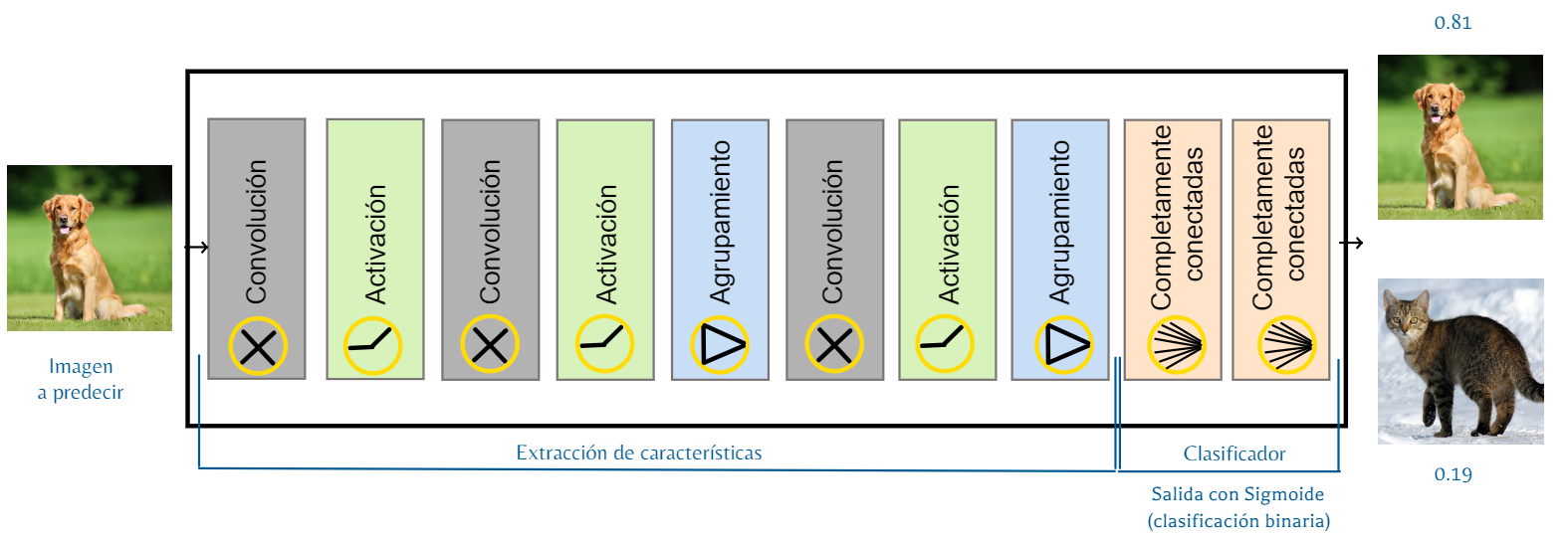
As the previous image shows, the data flow starts with the input image, which passes through several convolutional and activation layers to extract features, followed by pooling layers to reduce dimensionality. Finally, the extracted features are flattened and passed through fully connected layers to perform the final classification.

But, do all CNN networks have to follow the specific scheme shown? 😲

No, there is no single fixed recipe!

The specific architecture can vary depending on the problem being addressed, the nature of the data, and the model's objectives. Some CNNs may include additional layers such as normalization layers (Batch Normalization), dropout layers to prevent overfitting, or even more complex structures like residual blocks (ResNet) or Inception modules.

The key is to experiment with different architectures and evaluate their performance on the specific dataset to find the configuration that works best for the problem at hand.

And guess what? Optuna can help you with this too, simply by treating each layer as another hyperparameter to optimize. In the hands-on section, I'll show you a brief example of this.

In summary, a CNN transforms an image into a decision, going from pixels to features and from features to predictions. To better understand how these networks are built and trained, in the next section we will see a practical example with Keras.

Keras, the tool

Before starting with the practical part, let's make a brief stop to understand what Keras is, one of the most used libraries for creating deep learning models. Before continuing, I consider it important to mention that Keras v3 offers 3 ways to create models, you can check the complete detail on the Keras website. However, as a summary, let me briefly tell you the difference between them:

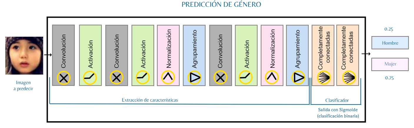
1. Sequential API: Simple way to stack layers, supports a single input and output.

   Example: Predict the gender (1 output) of a person from their facial image (1 input).

   
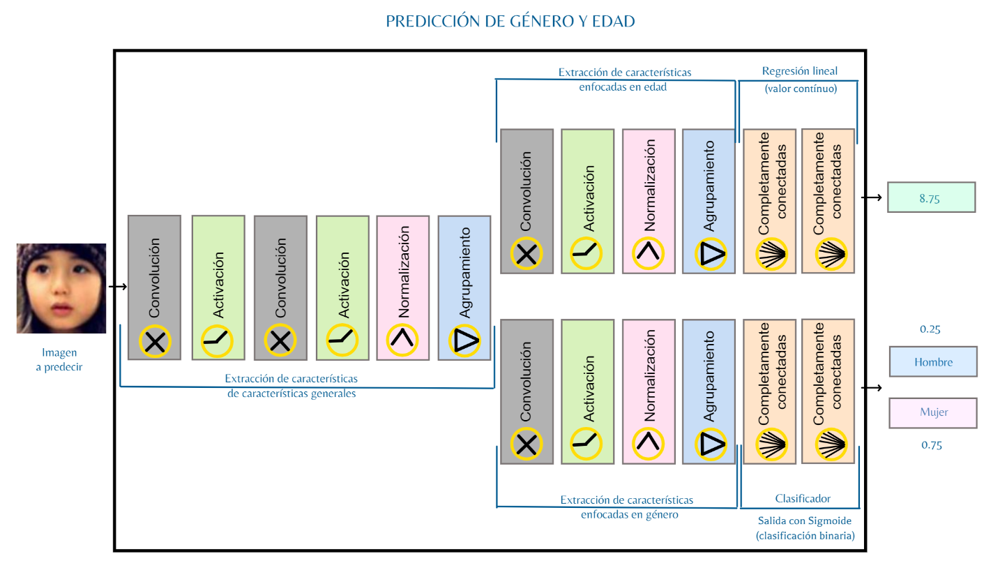
2. Functional API: Allows more customizable architectures with multiple inputs and outputs.

   Example: Predict the gender and age (2 outputs) of a person from their facial image (1 input).

   
3. Model subclassing: Allows creating dynamic architectures that adapt to requirements where greater control is needed over data flow and network logic depending on the input type.

   Example: Add convolutional and pooling layers conditionally, depending on the size of the input image. If the image is large, add more layers to extract more features; if it's small, use fewer layers to avoid computational overhead. You can understand it as conditional flow logic within the network architecture that enhances the capabilities of the 2 previous architectures. This approach is frequently used in research architectures or when full control over the model's internal flow is sought.

As in this example we are going to create an architecture that will generate two output predictions (age and gender), we will use the Keras Functional API. You can follow the notebook available on Google Colab.

Hands-on time

Now that we understand the three ways to build models with Keras, it's time to get hands-on. In this section, we will implement step by step a convolutional neural network using the Functional API, one based on what we used in the gender and age prediction scheme.

The objective will be to reproduce the complete flow: from loading data to generating predictions.

Importing required libraries

First, we import the required libraries for this exercise. We will use Keras within the TensorFlow ecosystem, as it is currently the recommended way. Additionally, we will use NumPy, Matplotlib, and OpenCV for image manipulation and visualization.

Additionally, since we are in Google Colab, we also import drive from Google Colab and os to mount Google Drive and access files.

 # System libraries
import os
import random

# Libraries for processing
import numpy as np
import tensorflow as tf
from tensorflow import keras
from tensorflow.keras import layers
from tensorflow.keras.regularizers import l2
from tensorflow.keras.utils import plot_model

# Libraries for visualization
import cv2
import matplotlib.pyplot as plt

# Library to mount Google Drive (only in Google Colab)
from google.colab import drive

With these dependencies ready, we now have everything needed to define the work environment.

Variable definition

Next, we define some variables that we will use throughout the notebook. These include the Google Drive mount path, the number of images to display, the dataset path, the path to save trained models, batch size, image size, number of epochs, channels, and the percentage of data to use for training.

MOUNT_POINT = "/content/drive" # Google Drive mount point
DATASET_PATH = "/content/drive/MyDrive/train_val" # Path to access the dataset
FOLDER_MODELS = "/content/drive/MyDrive/models" # Path to save trained models
IMAGES_TO_DISPLAY = 20 # Number of images to display in visualization
BATCH_SIZE = 32 # Batch size for training
IMAGE_SIZE = 128 # Size to which images will be resized
EPOCHS = 10 # Number of epochs for training
NUM_CHANNELS = 3 # Number of image channels
TRAINING_PERCENTAGE = 0.8 # Percentage of data to use for training

These variables will help us keep the code organized and facilitate any adjustments we need to make in the future.

Mount Google Drive

Since the data is stored in Google Drive, the next step is to mount Google Drive in the Colab environment to access the files.

drive.mount(MOUNT_POINT)

When executing this, the browser will ask for authorization to access Google Drive; simply follow the on-screen instructions.

Visualizing a sample of images

This step is optional but recommended to better understand the dataset we will be working with.

Load images to tensorflow dataframe

Now that we have access to the data, the next step is to load a sample of images from the dataset to visualize them and better understand what type of images we are handling.

file_names = os.listdir(DATASET_PATH) # List all files in the dataset directory
random_images = random.sample(file_names, IMAGES_TO_DISPLAY) # Randomly select images
images, age_labels, gender_labels = [], [], [] # Create lists for images and labels

for image in random_images: # Iterate over the selected images
    labels = image.split('_') # Extract age and gender labels from the filename delimited by '_'
    image = cv2.imread(os.path.join(DATASET_PATH, image)) # Read the image using OpenCV
    image = cv2.cvtColor(image, cv2.COLOR_BGR2RGB) # Convert from BGR to RGB

    age_label = int(labels[0]) # Age is the first part of the filename
    gender_label = int(labels[1]) # Gender is the second part of the filename

    age_labels.append(age_label) # Add the age label to the list
    gender_labels.append(gender_label) # Add the gender label to the list
    images.append(image) # Add the image to the list

# Convert lists to NumPy arrays to load them into tensorflow dataset
images_sample = np.array(images, dtype=np.int32)
age_sample = np.array(age_labels, dtype=np.int32)
gender_sample = np.array(gender_labels, dtype=np.int32)

# Create a tensorflow dataset object based on the samples
sample_ds = tf.data.Dataset.from_tensor_slices((images_sample, age_sample, gender_sample))
sample_ds = sample_ds.shuffle(len(images_sample)).batch(BATCH_SIZE).prefetch(tf.data.AUTOTUNE)

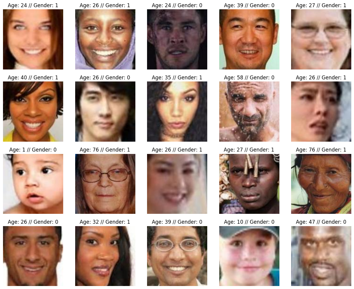
Here, we randomly select a set of images from the dataset directory, read them, and convert them to RGB format (since OpenCV reads them in BGR format by default). Additionally, we extract the age and gender labels from the file names, as we know the name format is age_gender_race_unique-id.jpg.

For example, a file named 25_0_3_123432323235.jpg indicates that the person in the image is 25 years old and female (0). Similarly, a file named 30_1_4_23231267890.jpg indicates that the person is 30 years old and male (1).

Finally, we convert the image and label lists into NumPy arrays and create a tf.data.Dataset to facilitate data manipulation and processing.

Preview of loaded images

Finally, we visualize the loaded images along with their age and gender labels to ensure they have been loaded correctly.

plt.figure(figsize=(15, 12)) # Configure the figure size
for image, age, gender in sample_ds.take(1):  # Take a batch from the dataset
    for i in range(IMAGES_TO_DISPLAY): # Iterate over the images in the batch
        ax = plt.subplot(4, 5, i + 1) # Create a subplot for each image
        plt.imshow(np.array(image[i]).astype("uint8")) # Show the image
        plt.title(f"Age: {int(age[i])} // Gender: {int(gender[i])}") # Print the title with age and gender
        plt.axis("off")

As we can observe, the images have been loaded correctly, and the age and gender labels match the displayed images. This confirms that we are ready to proceed with preprocessing and model training.

Partitioning the dataset

Now that we have visualized a sample of the images, the next step is to divide the dataset into training and validation sets. This is crucial for evaluating the model's performance during training and ensuring we don't fall into overfitting.

all_image_files = [file for file in os.listdir(DATASET_PATH) if file.lower().endswith(('.jpg'))] # List all image files in the dataset directory
random.seed(0) # Set a seed for shuffle reproducibility
random.shuffle(all_image_files) # Randomly shuffle the image files

total_images = len(all_image_files) # Count the total number of images
train_end = int(total_images * TRAINING_PERCENTAGE) # Calculate the index to split the dataset

# Separate files into training and validation sets
train_image_files = all_image_files[:train_end] # Image files for training
val_image_files = all_image_files[train_end:] # Image files for validation 

Here, we list all image files in the dataset directory and shuffle them randomly to ensure the split is representative. Then, we calculate the index to divide the dataset according to the defined percentage for training (80% in this case) and separate the files into training and validation sets.

Data segmentation

Next, we define a function to load the images and their labels (age and gender) from the file names. This function will read each image, convert it to RGB format, normalize it, and extract the age and gender labels from the file name.

Read and process images and labels

The load_images_labels function takes as input the dataset path and a list of file names. It returns three NumPy arrays: one with the processed images, another with age labels, and another with gender labels.

# Define a function to load images and their labels (edad y género) desde los nombres de archivo
def load_images_labels(dataset_path, filenames):
  images, age_labels, gender_labels = [], [], [] # Create lists for images and labels

  for current_file_name in filenames: # Se itera sobre los nombres de archivo proporcionados
    image = cv2.imread(os.path.join(dataset_path, current_file_name)) # Read the image using OpenCV
    image = cv2.cvtColor(image, cv2.COLOR_BGR2RGB) # Convert from BGR to RGB
    image = image / 255.0  # Normalize the image to [0, 1] as recommended practice
    labels = current_file_name.split('_') # Extraemos las etiquetas de edad y género del nombre del archivo
    age_label = int(labels[0]) # Age is the first part of the filename
    gender_label = int(labels[1]) # Gender is the second part of the filename

    age_labels.append(age_label) # Add the age label to the list
    gender_labels.append(gender_label) # Add the gender label to the list
    images.append(image) # Add the image to the list

  # Convert lists to NumPy arrays to load them into tensorflow dataset
  images = np.array(images) 
  age_labels = np.array(age_labels)
  gender_labels = np.array(gender_labels)
  
  return images, age_labels, gender_labels

Load data into memory

Now, we use the function defined earlier to load the images and their labels for both the training and validation sets.

# Call the function to load training images and labels into memory
train_images, train_age, train_gender = load_images_labels(DATASET_PATH, train_image_files)

# Call the function to load validation images and labels into memory
val_images, val_age, val_gender = load_images_labels(DATASET_PATH, val_image_files)

Create TensorFlow dataset objects

Finally, we convert the image and label arrays into tf.data.Dataset objects to facilitate their manipulation during model training. These objects allow efficient data handling, including operations such as shuffling, batching, and prefetching to optimize performance during training.

# Create a tensorflow dataset object based on training images and labels
train_ds = tf.data.Dataset.from_tensor_slices(({"my_images_input": train_images}, {"age_output":train_age, "gender_output":train_gender}))
train_ds = train_ds.shuffle(len(train_images)).batch(BATCH_SIZE).prefetch(tf.data.AUTOTUNE)

# Create a tensorflow dataset object based on validation images and labels
val_ds = tf.data.Dataset.from_tensor_slices(({"my_images_input": val_images}, {"age_output":val_age, "gender_output":val_gender}))
val_ds = val_ds.shuffle(len(val_images)).batch(BATCH_SIZE).prefetch(tf.data.AUTOTUNE)

Data augmentation

Although this concept was not mentioned during the theory covered, data augmentation is a crucial technique in training deep learning models, especially when working with limited datasets.

It consists of applying random transformations to training images to create additional variations, which helps improve the model's generalization (ability to predict correctly on unseen data), avoiding overfitting.

# Define a function to apply data augmentation to images
def data_augmentation(images):
    for layer in data_augmentation_layers:
        images = layer(images)
    return images

# Define the data augmentation techniques we will apply
data_augmentation_layers = [
    layers.RandomFlip("horizontal"), # Flip horizontally
    layers.RandomRotation(0.1), # Rotate randomly up to 10%
    layers.RandomZoom(0.14) # Apply random zoom up to 14%
]

In this case, we have defined three augmentation techniques: horizontal flip, random rotation, and random zoom. These transformations will be applied to the training images during the model training process, helping to create a more diverse and robust dataset.

The specific rotation and zoom values are also hyperparameters that can be adjusted to optimize the model's performance. So they can be included in the optimization process with Optuna as we mentioned earlier.

You can find all available augmentation techniques in the Keras documentation.

Model architecture definition

Now that we have prepared the data, it's time to define the architecture of our convolutional neural network (CNN). We will use the Keras Functional API to create a model with multiple outputs, one to predict age and another to predict gender.

Main branch layers of the model

We start by defining the model input, which will be an image of size 128x128 with 3 color channels (RGB). Then, we apply the data augmentation techniques defined earlier.

Next, we define the main CNN architecture, which consists of several blocks of convolutional layers followed by batch normalization layers and pooling layers to extract relevant features from the images.

Each layers.Conv2D layer represents a convolutional layer, where the values inside the parentheses are the hyperparameters mentioned earlier. For example, in the first convolutional layer, we use 64 filters of size 3x3 with the ReLU activation function and "same" padding to maintain the spatial dimensions of the image. This same idea applies to the other layers in the network.

But did you notice that we mentioned ReLU as a hyperparameter of the convolutional layer?

This is a separate layer according to what we saw in the theory covered, but in Keras it is included within the definition of the convolutional layer as another hyperparameter.

Another important point we must mention is that the values at the end ((x) / (branch_gender) / (branch_age)) of each layer (Conv2D, MaxPooling2D, Flatten, Dense, Dropout) are the output of the previous layer, that is, the layer on which the changes of the next layer are applied.

Example: The output of the Conv2D layer (x_output_1) is used as input for the BatchNormalization layer:
x_salida_1 = layers.Conv2D(...)(x_salida_0)
x_salida_2 = layers.BatchNormalization(...)(x_salida_1)

image_inputs = keras.Input(shape=(IMAGE_SIZE, IMAGE_SIZE, NUM_CHANNELS), name="my_images_input") # Define the model input
x = data_augmentation(image_inputs) # Apply data augmentation

# Define the main CNN architecture
## Feature extraction block 1
x = layers.Conv2D(64, (3, 3), activation="relu", padding="same")(x) # First convolutional layer
x = layers.BatchNormalization()(x) # Batch normalization
x = layers.Conv2D(64, (3, 3), activation="relu", padding="same")(x) # Second convolutional layer
x = layers.BatchNormalization()(x) # Batch normalization
x = layers.MaxPooling2D((2, 2))(x) # Pooling layer

## Feature extraction block 2
x = layers.Conv2D(64, (3, 3), activation="relu", padding="same")(x) # Third convolutional layer
x = layers.BatchNormalization()(x) # Batch normalization
x = layers.Conv2D(64, (3, 3), activation="relu", padding="same")(x) # Fourth convolutional layer
x = layers.BatchNormalization()(x) # Batch normalization
x = layers.MaxPooling2D((2, 2))(x) # Pooling layer

## Feature extraction block 3
x = layers.Conv2D(512, (3, 3), activation="relu", padding="same")(x) # Fifth convolutional layer
x = layers.BatchNormalization()(x) # Batch normalization
x = layers.MaxPooling2D((2, 2))(x) # Pooling layer

The output of this section will serve as input for the two branches of the model, one to predict age and another to predict gender.

Age branch layers

Next, we define the model branch responsible for predicting age. This branch takes the output of the main architecture and goes through several blocks of convolutional and fully connected layers before generating the final age prediction.

# Branch for age prediction
## Feature extraction block for age
branch_age = layers.Conv2D(128, (3, 3), activation="relu", padding="same", kernel_regularizer=l2(0.01))(x) # First convolutional layer
branch_age = layers.BatchNormalization()(branch_age) # Batch normalization
branch_age = layers.Conv2D(128, (3, 3), activation="relu", padding="same", kernel_regularizer=l2(0.01))(branch_age) # Second convolutional layer
branch_age = layers.BatchNormalization()(branch_age) # Batch normalization
branch_age = layers.MaxPooling2D((2, 2))(branch_age) # Pooling layer

## Block for age prediction
branch_age = layers.Flatten()(branch_age) # Flattening
branch_age = layers.Dense(128, activation="relu")(branch_age) # Fully connected layer
branch_age = layers.Dropout(0.45)(branch_age) # Dropout layer to prevent overfitting
age_output = layers.Dense(1, activation="linear", name="age_output")(branch_age) # Output for age prediction

The output of this branch is a single neuron with linear activation, suitable for a regression problem like age prediction.

Gender branch layers

Now, we define the model branch responsible for predicting gender. Similar to the age branch, this branch also takes the output of the main architecture and goes through several blocks of convolutional and fully connected layers before generating the final gender prediction.

# Branch for gender prediction
## Feature extraction block for gender
branch_gender = layers.Conv2D(128, (3, 3), activation="relu", padding="same")(x) # First convolutional layer
branch_gender = layers.BatchNormalization()(branch_gender) # Batch normalization
branch_gender = layers.Conv2D(128, (3, 3), activation="relu", padding="same")(branch_gender) # Second convolutional layer
branch_gender = layers.BatchNormalization()(branch_gender) # Batch normalization
branch_gender = layers.MaxPooling2D((2, 2))(branch_gender) # Pooling layer

## Block for gender prediction
branch_gender = layers.Flatten()(branch_gender) # Flattening
branch_gender = layers.Dense(128, activation="relu")(branch_gender) # Fully connected layer
branch_gender = layers.Dropout(0.26871378401366075)(branch_gender) # Dropout layer to prevent overfitting
gender_output = layers.Dense(1, activation="sigmoid", name="gender_output")(branch_gender) # Output for gender prediction

The output of this branch is a single neuron with sigmoid activation, suitable for a binary classification problem like gender prediction (male or female).

Model inputs and outputs

Finally, we define the complete model by specifying the inputs and outputs. We use the keras.Model class to create a model with multiple outputs, one for age and another for gender.

# Define the model with multiple inputs and outputs
model = keras.Model(
    inputs=[image_inputs],
    outputs=[age_output, gender_output]
)

Model architecture summary

We can print a summary of the model architecture to verify that everything is defined correctly. This will show us the model layers, the number of trainable and non-trainable parameters, and the shape of the outputs of each layer. You can see the diagram in the Colab of this article.

model.summary() # Print the model summary

Model graph

We can also visualize the model architecture as a graph, which helps us better understand the structure and connections between the different layers. You can see the graph in the Colab of this article.

plot_model(model, show_shapes=True, dpi=100) # Visualize the model architecture

Hyperparameter definition

Before training the model, we need to define several important hyperparameters that will influence the training process and the final performance of the model. These include loss functions, loss weights for each task (age and gender), the optimizer, evaluation metrics, and training callbacks.

Age and gender loss weights

Since we are addressing a multi-task learning problem, it is important to assign appropriate weights to the losses of each task. In this case, we have decided to assign a slightly higher weight to the age loss compared to the gender loss, as age prediction can be more challenging and critical in this context.

loss_weight_gender = 0.6940071116394927 # Weight for gender loss
loss_weight_age = 1.0 - loss_weight_gender # Weight for age loss
loss_weights = {
    "age_output": loss_weight_age,
    "gender_output": loss_weight_gender
}

Optimizer, metrics and training callbacks

We will use the Adam optimizer, which is widely used in deep learning tasks due to its ability to adapt to different learning rates during training. Additionally, we will define the loss functions and evaluation metrics for each task.

optimizer = keras.optimizers.Adam(learning_rate=1e-4) # Define the Adam optimizer with a learning rate of 0.0001

# Compile the model with multiple losses and metrics
model.compile(
    optimizer=optimizer,
    loss={"age_output": keras.losses.Huber(delta=5.0), "gender_output": "binary_crossentropy"},
    loss_weights=loss_weights,
    metrics={"age_output": "mae", "gender_output": "accuracy"}
)

# Define callbacks for training
CALLBACKS = [
    tf.keras.callbacks.EarlyStopping(monitor='val_loss', min_delta=0.01, patience=10, mode='auto', restore_best_weights=True),
    tf.keras.callbacks.ReduceLROnPlateau(monitor='val_loss', factor=0.5, patience=7, min_lr=1e-6, verbose=0),
]

The defined callbacks include EarlyStopping to stop training if the validation loss does not improve after a certain number of epochs, and ReduceLROnPlateau to reduce the learning rate if the validation loss stagnates.

Model training

Now, we are ready to train the model using the training and validation datasets that we prepared earlier. The training process will involve feeding the images and labels to the model in batches, adjusting the neural network weights through backpropagation, and evaluating the model's performance on the validation set after each epoch.

# Train the model
history = model.fit(train_ds, # Training dataset
                    batch_size=BATCH_SIZE, # Batch size
                    epochs=EPOCHS, # Number of epochs
                    callbacks=CALLBACKS, # Callbacks defined earlier
                    validation_data=val_ds, # Validation dataset
                    verbose=1 # Show training progress
                    )

Save the trained model

Once the model has been trained, it is important to save the weights and architecture of the model so they can be reused later without needing to retrain from scratch. Keras provides a simple way to save and load complete models using the HDF5 format or TensorFlow's native format.

# Create a directory to save the model if it does not exist
if not os.path.exists(FOLDER_MODELS):
    os.mkdir(FOLDER_MODELS)

model.save(FOLDER_MODELS+'/age-gender.keras') # Save the model

Training and validation metrics

During model training, it is useful to visualize performance metrics on both the training and validation sets. This allows us to monitor the model's progress and detect possible problems such as overfitting or underfitting.

# Visualize training and validation metrics
fig = plt.figure(figsize=(15, 10))
fig.add_subplot(2,2,1)
plt.plot(history.history['gender_output_loss'], label='train gender loss')
plt.plot(history.history['val_gender_output_loss'], label='val gender loss')
plt.legend()
plt.grid(True)
plt.ylim([0,1.0])
plt.xlabel('epoch')

fig.add_subplot(2,2,2)
plt.plot(history.history['gender_output_accuracy'], label='train gender accuracy')
plt.plot(history.history['val_gender_output_accuracy'], label='val gender accuracy')
plt.legend()
plt.grid(True)
plt.ylim([0,1.0])
plt.xlabel('epoch')

fig.add_subplot(2,2,3)
plt.plot(history.history['age_output_loss'], label='train age loss')
plt.plot(history.history['val_age_output_loss'], label='val age loss')
plt.legend()
plt.grid(True)
plt.xlabel('epoch')

fig.add_subplot(2,2,4)
plt.plot(history.history['age_output_mae'], label='train age mae')
plt.plot(history.history['val_age_output_mae'], label='val age mae')
plt.legend()
plt.grid(True)
plt.xlabel('epoch')

Model evaluation

Finally, we evaluate the model's performance on the validation set using the model.evaluate() method. This provides us with an objective evaluation of the model on data not seen during training.

print(model.evaluate(val_ds)) # Evaluate the model on the validation set

Demo

Because explaining it is good, but showing it is better, I have created an interactive demo where you can upload a photo and the trained model will tell you the estimated age and gender. You can try it below:

Images are not stored or sent to external servers; they are processed in Hugging Face Space.

Closing

In this article, we have covered the complete process of building and training a convolutional neural network (CNN) from scratch using Keras and TensorFlow. Throughout the development, we addressed data preparation and preprocessing, architecture definition, model training, and final evaluation.

I hope this post has provided you with a solid understanding of how to build and train a CNN for computer vision tasks. I encourage you to experiment with different architectures, data augmentation techniques, and datasets to explore how each design decision impacts model performance.

Additionally, the interactive demo accompanying this article is supported in a zero-cost environment thanks to Hugging Face Spaces, a platform that allows you to deploy deep learning models for free and accessibly. This shows that today it is possible to share functional prototypes and deep learning experiments without relying on expensive infrastructure, making technology more accessible to everyone.

If you are interested in continuing to learn about concepts and practical cases in Machine Learning, Deep Learning, Computer Vision, and GenAI, I invite you to connect via LinkedIn and stay tuned for upcoming posts and projects in my portfolio. In future installments, we will also explore how to apply these technologies in cloud environments, using services from AWS, Google Cloud Platform, and Microsoft Azure for building, automating, and deploying AI solutions at scale.

Thank you for reading and happy deep learning!